Tutorial
Overview
scikit-mpe package allows you to extract N-dimensional minimal paths using existing speed data and starting/ending and optionally way points initial data.
Note
The package does not compute any speed data (a.k.a speed function). It is expected that the speed data was previously obtained/computed in some way.
The package can be useful for various engineering and image processing tasks. For example, the package can be used for extracting paths through tubular structures on 2-d and 3-d images, or shortest paths on a terrain map.
The package uses the fast marching method and ODE solver for extracting minimal paths.
Algorithm
The algorithm contains two main steps:
First, the travel time is computing from the given ending point (zero contour) to every speed data point using the fast marching method.
Second, the minimal path (travel time is minimizing) is extracting from the starting point to the ending point using ODE solver (Runge-Kutta for example) for solving the differential equation \(x_t = - \nabla (t) / | \nabla (t) |\)
If we have way points we need to perform these two steps for every interval between the starting point, the set of the way points and the ending point and concatenate the path pieces to the full path.
Quickstart
Let’s look at a simple example of how the algorithm works.
Note
We will use retina test image from scikit-image package as the test data for all examples.
First, we need a speed data (speed function). We can use one of the tubeness filters for computing speed data for our test data, sato filter for example.
from skimage.data import retina
from skimage.color import rgb2gray
from skimage.transform import rescale
from skimage.filters import sato

image_data = rescale(rgb2gray(retina()), 0.5)
speed_data = sato(image_data) + 0.05
speed_data[speed_data > 1.0] = 1.0

_, (ax1, ax2) = plt.subplots(1, 2)
ax1.imshow(image_data, cmap='gray')
ax1.set_title('source data')
ax1.axis('off')
ax2.imshow(speed_data, cmap='gray')
ax2.set_title('speed data')
ax2.axis('off')
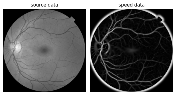
The speed data values must be in range [0.0, 1.0] and can be masked also.
where:
0.0 – zero speed (impassable)
1.0 – max speed
masked – impassable
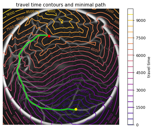
Second, let’s try to extract the minimal path for some starting and ending points using scikit-mpe package and plot it. Also we can plot travel time contours.
from skmpe import mpe

# define starting and ending points
start_point = (165, 280)
end_point = (611, 442)

path_info = mpe(speed_data, start_point, end_point)

# get computed travel time for given ending point and extracted path
travel_time = path_info.pieces[0].travel_time
path = path_info.path

nrows, ncols = speed_data.shape
xx, yy = np.meshgrid(np.arange(ncols), np.arange(nrows))

fig, ax = plt.subplots(1, 1)
ax.imshow(speed_data, cmap='gray', alpha=0.9)
ax.plot(path[:,1], path[:,0], '-', color=[0, 1, 0], linewidth=2)
ax.plot(start_point[1], start_point[0], 'or')
ax.plot(end_point[1], end_point[0], 'o', color=[1, 1, 0])
tt_c = ax.contour(xx, yy, travel_time, 20, cmap='plasma', linewidths=1.5)
ax.clabel(tt_c, inline=1, fontsize=9, fmt='%d')
ax.set_title('travel time contours and minimal path')
ax.axis('off')
cb = fig.colorbar(tt_c)
cb.ax.set_ylabel('travel time')
Advanced Usage
Initial Data
The initial data is storing and validating in InitialInfo class which inherited from
Pydantic BaseModel. The class checks speed data and points dimensions, boundaries and values.
Therefore, we cannot set an invalid data:
import numpy as np
from skmpe import InitialInfo

speed_data = np.zeros((100, 200))
start_point = (10, 300)  # out of bounds
end_point = (50, 60)

init_data = InitialInfo(
    speed_data=speed_data,
    start_point=start_point,
    end_point=end_point,
)
The code above is raising an exception:
Traceback (most recent call last):
  ...
    raise validation_error
pydantic.error_wrappers.ValidationError: 1 validation error for InitialInfo
start_point
  'start_point' (10, 300) coordinate 1 is out of 'speed_data' bounds [0, 200). (type=value_error)
We can use InitialInfo explicity in mpe() function:
from skmpe import InitialInfo, mpe

init_data = InitialInfo(...)
result = mpe(init_data)
Also in most cases we can use the second mpe() function signature without using InitialInfo explicity:
from skmpe import mpe

...

result = mpe(speed_data, start_point, end_point)
Parameters
The algorithm parameters are storing and validating in Parameters class.
We can use this class directly, or we can use parameters() context manager for manage parameters.
Also default_parameters() function returns the instance with default parameters:
>>> from skmpe import default_parameters
>>> print(default_parameters())

travel_time_spacing=1.0
travel_time_order=<TravelTimeOrder.first: 1>
travel_time_cache=False
ode_solver_method=<OdeSolverMethod.RK45: 'RK45'>
integrate_time_bound=10000.0
integrate_min_step=0.0
integrate_max_step=4.0
dist_tol=0.001
max_small_dist_steps=100
Important Parameters
The following parameters may be important in some cases:
travel_time_order – the order of the fast-marching computation method. 2 is more accurate, but it is slower. By default it is 1. Use
TravelTimeOrderenum for this parametertravel_time_cache – if we set way points we can use cached travel time. For example if we set one way point we can compute travel time once for this way point as source point. By default it is False.
ode_solver_method – we can use some ODE methods for extracting path. Some methods may be work faster or more accurate on some speed data. Use
OdeSolverMethodenum for this parameter. By default it is Runge-Kutta 4/5 (RK45)integrate_time_bound – if we want to extract a long path we need to set a greater value for time bound. By default it is 10000
integrate_min_step, integrate_max_step – these options can be used to control of ODE solver steps. For example, lower value of
integrate_max_stepleads to lower the performance, but higher the accuracy.dist_tol – distance tolerance between steps for control path evolution. By default it is 0.001
max_small_dist_steps – the maximum number of small distance steps while path evolution. Too small steps will be ignore N-times by this parameter.
Using Parameters
We can set the custom parameter values by Parameters class or parameters() context manager.
Using class:
from skmpe import Parameters, mpe

my_parameters = Parameters(travel_time_cache=True, travel_time_order=1)
result = mpe(..., parameters=my_parameters)
Using context manager:
from skmpe import parameters, mpe

with parameters(travel_time_cache=True, travel_time_order=1):
    # the custom parameters will be used automatically
    result = mpe(...)
Results
The whole extracted path results are storing in PathInfoResult class (named tuple).
The instance of this class is returning from mpe() function. The pieces of the path
(in the case with way points) are storing in PathInfo class.
PathInfoResult object contains:
path – the whole extracted path in numpy array MxN where M is the number of points and N is dimension
pieces – the list of extracted path pieces between start/end or way points in PathInfo instances. If we do not use way points, pieces list will be contain one piece.
PathInfo object contains:
path – the extracted path piece in numpy array MxN where M is the number of points and N is dimension
start_point – the starting point
end_point – the ending point
travel_time – the computed travel time data for given speed data
extraction_result – the raw extraction result in
PathExtractionResultinstance. This data is returning fromMinimalPathExtractorclass (low-level API). The data contains additional info about extracted path and info about extracting process. This data may be useful for debugging.reversed – The flag indicates that the path piece is reversed. This is relevant when using
travel_time_cache == Trueparameter.
Low-level API
If you need full control over the extracting process, you can use MinimalPathExtractor class.
The class is used inside mpe() function for extracting the pieces of path.
Here is a simple example of usage:
from skmpe import MinimalPathExtractor, Parameters

speed_data = ...
start_point = ...
end_point = ...
parameters = Parameters(...)  # optional, also we can use 'parameters' context manager

# Create the instance and compute travel time data
mpe = MinimalPathExtractor(speed_data, end_point, parameters)

# get computed travel time data
travel_time = mpe.travel_time

# get phi (zero contour for given end_point)
phi = mpe.phi

# extract path from start_point to end_point
# it returns PathExtractionResult instance
extracting_result = mpe(start_point)

# the list of path points
path_points = extracting_result.path_points

# the list of integrate time values in every path point
path_integrate_times = extracting_result.path_integrate_times

# the list of travel time values in every path point
path_travel_times = extracting_result.path_travel_times

# the number of ODE solver steps
step_count = extracting_result.step_count

# the number of right hand function evaluations in ODE solver
func_eval_count = extracting_result.func_eval_count